
!pip install matplotlib s3fs "xarray[io]"
import zarr
import numpy as np
import xarray as xr
import matplotlib.pyplot as plt
from matplotlib.colors import LogNorm
from scipy.signal import stft
Level 2 Data#
In this notebook we demonstrate the variety of different data available in the FAIR MAST dataset. In this example we are using level 2 MAST data, which includes cropping, interpolation, calibration, etc. of each signal, as well as mapping each diagnostic group try and follow IMAS naming convetions. The level 2 data is well-indexed data and follows the FAIR principles. Shots are also filtered using the plasma current to remove shots which were only used for testing, comissioning, machine calibration etc.
First we need to connect to the remote S3 storage bucket to access the data. Each shot from MAST is stored as a seperate Zarr file.
Using fsspec and xarray we can remotely read data directly over the web. In the example below we also turn on local file caching, allowing us to avoid reading over the network multiple times.
shot_id = 30421

endpoint_url = 'https://s3.echo.stfc.ac.uk'
url = f's3://mast/level2/shots/{shot_id}.zarr'

# Get a handle to the remote file
store = zarr.storage.FsspecStore.from_url(
    url,
    storage_options=dict(
        protocol='simplecache',
        target_protocol="s3",
        cache_storage='.cache',
        target_options=dict(
            anon=True, endpoint_url=endpoint_url, asynchronous=True
        )
    )
)
Summary Profiles#
The summary group provides a collection of general physics quantities for an experiment.
profiles = xr.open_zarr(store, group='summary')

plot_1d_profiles(profiles)
profiles
<xarray.Dataset> Size: 49kB
Dimensions:              (time: 767)
Coordinates:
  * time                 (time) float64 6kB -0.1 -0.099 -0.098 ... 0.665 0.666
    shot_id              int64 8B ...
Data variables:
    greenwald_density    (time) float64 6kB ...
    ip                   (time) float64 6kB ...
    line_average_n_e     (time) float64 6kB ...
    neutron_rates_total  (time) float64 6kB ...
    power_nbi            (time) float64 6kB ...
    power_ohm            (time) float64 6kB ...
    power_radiated       (time) float64 6kB ...
Attributes:
    name:          summary
    description:   Summary of physics quantities from a simulation or an expe...
    imas:          summary
    license_name:  Creative Commons 4.0 BY-SA
    license_url:   https://creativecommons.org/licenses/by-sa/4.0/
    ingested_at:   2026-09-24T17:10:53Z
    commit_url:    https://github.com/ukaea/fair-mast-ingestion/tree/ed6ea4e2...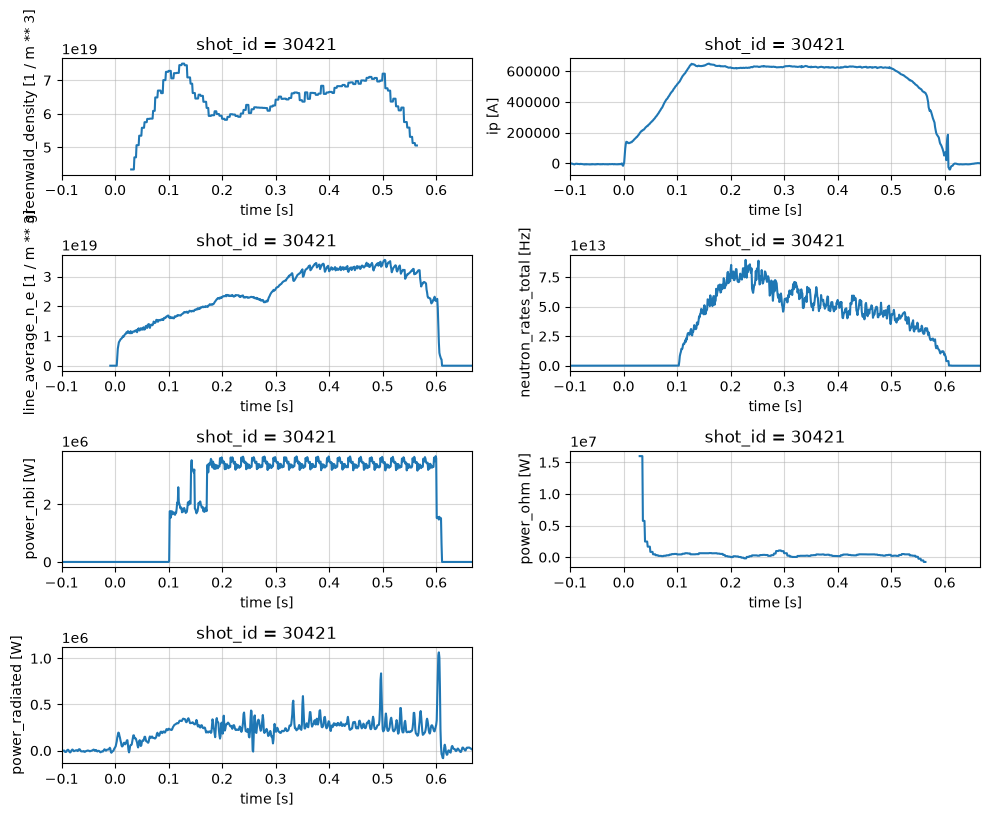
Pulse Schedule#
profiles = xr.open_zarr(store, group='pulse_schedule')

fig, axes = plt.subplots(2, 1, figsize=(10, 5))
axes = axes.flatten()
profiles['i_plasma'].plot(x='time', ax=axes[0])
profiles['n_e_line'].plot(x='time', ax=axes[1])


for ax in axes:
    ax.grid('on', alpha=0.5)
plt.tight_layout()

profiles
<xarray.Dataset> Size: 490kB
Dimensions:   (time: 15305)
Coordinates:
  * time      (time) float64 122kB -0.1 -0.09995 -0.0999 ... 0.6652 0.6652
    shot_id   int64 8B ...
Data variables:
    i_plasma  (time) float64 122kB ...
    n_e_line  (time) float64 122kB ...
    z_ref     (time) float64 122kB ...
Attributes:
    name:          pulse_schedule
    description:   Description of Pulse Schedule, described by subsystems wav...
    imas:          pulse_schedule
    license_name:  Creative Commons 4.0 BY-SA
    license_url:   https://creativecommons.org/licenses/by-sa/4.0/
    ingested_at:   2026-09-24T17:10:51Z
    commit_url:    https://github.com/ukaea/fair-mast-ingestion/tree/ed6ea4e2...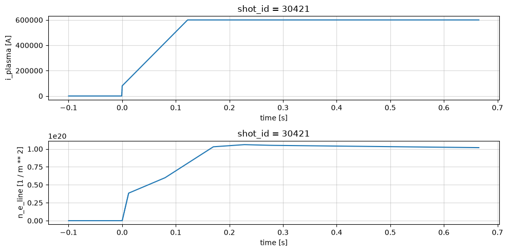
Magnetics#
Magnetic diagnostics for equilibrium identification and plasma shape control.
profiles = xr.open_zarr(store, group='magnetics')

fig, axes = plt.subplots(4, 3, figsize=(8, 10))
axes = axes.flatten()

profiles['b_field_pol_probe_ccbv_field'].plot.line(x='time', ax=axes[0], add_legend=False)
profiles['b_field_pol_probe_obv_field'].plot.line(x='time', ax=axes[1], add_legend=False)
profiles['b_field_pol_probe_obr_field'].plot.line(x='time', ax=axes[2], add_legend=False)


profiles['b_field_pol_probe_omv_voltage'].plot.line(x='time_mirnov', ax=axes[3], add_legend=False)
profiles['b_field_pol_probe_cc_field'].plot.line(x='time_mirnov', ax=axes[4], add_legend=False)
profiles['b_field_tor_probe_cc_field'].plot.line(x='time_mirnov', ax=axes[5], add_legend=False)

profiles['b_field_tor_probe_saddle_field'].plot.line(x='time_saddle', ax=axes[6], add_legend=False)
profiles['b_field_tor_probe_saddle_voltage'].plot.line(x='time_saddle', ax=axes[7], add_legend=False)
profiles['b_field_tor_probe_omaha_voltage'].plot.line(x='time_omaha', ax=axes[8], add_legend=False)

profiles['flux_loop_flux'].plot.line(x='time', ax=axes[9], add_legend=False)
profiles['ip'].plot.line(x='time', ax=axes[10], add_legend=False)

for ax in axes[:11]:
    ax.grid('on', alpha=0.5)

# remove the unused 12th axis in the 4x3 grid
fig.delaxes(axes[11])

plt.tight_layout()

profiles
<xarray.Dataset> Size: 109MB
Dimensions:                                      (
                                                  b_field_pol_probe_cc_channel: 5,
                                                  time_mirnov: 382601,
                                                  b_field_pol_probe_cc_geometry_channel: 40,
                                                  b_field_pol_probe_ccbv_channel: 40,
                                                  time: 3827,
                                                  ...
                                                  coordinate: 28,
                                                  b_field_tor_probe_saddle_m_geometry_channel: 12,
                                                  b_field_tor_probe_saddle_u_geometry_channel: 12,
                                                  b_field_tor_probe_saddle_voltage_channel: 12,
                                                  flux_loop_channel: 15,
                                                  flux_loop_geometry_channel: 46)
Coordinates: (12/26)
  * b_field_pol_probe_cc_channel                 (b_field_pol_probe_cc_channel) StringDType() 80B ...
  * time_mirnov                                  (time_mirnov) float64 3MB -0...
  * b_field_pol_probe_cc_geometry_channel        (b_field_pol_probe_cc_geometry_channel) StringDType() 640B ...
  * b_field_pol_probe_ccbv_channel               (b_field_pol_probe_ccbv_channel) StringDType() 640B ...
  * time                                         (time) float64 31kB -0.1 ......
  * b_field_pol_probe_ccbv_geometry_channel      (b_field_pol_probe_ccbv_geometry_channel) StringDType() 640B ...
    ...                                           ...
  * b_field_tor_probe_saddle_m_geometry_channel  (b_field_tor_probe_saddle_m_geometry_channel) StringDType() 192B ...
  * b_field_tor_probe_saddle_u_geometry_channel  (b_field_tor_probe_saddle_u_geometry_channel) StringDType() 192B ...
  * b_field_tor_probe_saddle_voltage_channel     (b_field_tor_probe_saddle_voltage_channel) StringDType() 192B ...
  * flux_loop_channel                            (flux_loop_channel) StringDType() 240B ...
  * flux_loop_geometry_channel                   (flux_loop_geometry_channel) StringDType() 736B ...
    shot_id                                      int64 8B 30421
Data variables: (12/46)
    b_field_pol_probe_cc_field                   (b_field_pol_probe_cc_channel, time_mirnov) float64 15MB ...
    b_field_pol_probe_cc_phi                     (b_field_pol_probe_cc_geometry_channel) float64 320B ...
    b_field_pol_probe_cc_r                       (b_field_pol_probe_cc_geometry_channel) float64 320B ...
    b_field_pol_probe_cc_z                       (b_field_pol_probe_cc_geometry_channel) float64 320B ...
    b_field_pol_probe_ccbv_field                 (b_field_pol_probe_ccbv_channel, time) float64 1MB ...
    b_field_pol_probe_ccbv_length                (b_field_pol_probe_ccbv_geometry_channel) float64 320B ...
    ...                                           ...
    b_field_tor_probe_saddle_u_z                 (b_field_tor_probe_saddle_u_geometry_channel, coordinate) float64 3kB ...
    b_field_tor_probe_saddle_voltage             (b_field_tor_probe_saddle_voltage_channel, time_saddle) float64 4MB ...
    flux_loop_flux                               (flux_loop_channel, time) float64 459kB ...
    flux_loop_r                                  (flux_loop_geometry_channel) float64 368B ...
    flux_loop_z                                  (flux_loop_geometry_channel) float64 368B ...
    ip                                           (time) float64 31kB -864.2 ....
Attributes:
    name:          magnetics
    description:   Magnetic diagnostics for equilibrium identification and pl...
    imas:          magnetics
    license_name:  Creative Commons 4.0 BY-SA
    license_url:   https://creativecommons.org/licenses/by-sa/4.0/
    ingested_at:   2026-09-24T17:15:15Z
    commit_url:    https://github.com/ukaea/fair-mast-ingestion/tree/ed6ea4e2...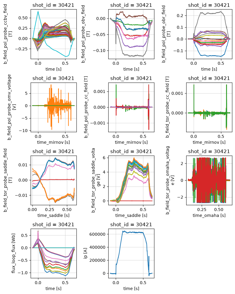
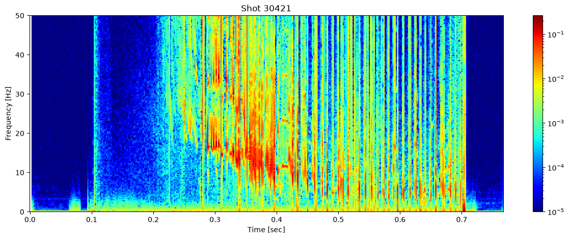
Looking at the spectrogram of one of the mirnov coils can show us information about the MHD modes. Here we see several mode instabilities occuring before the plasma is lost.
ds = profiles['b_field_pol_probe_omv_voltage'].isel(b_field_pol_probe_omv_channel=1)
# Parameters to limit the number of frequencies
nperseg = 2000  # Number of points per segment
nfft = 2000  # Number of FFT points

# Compute the Short-Time Fourier Transform (STFT)
sample_rate = 1/(ds.time_mirnov[1] - ds.time_mirnov[0])
f, t, Zxx = stft(ds, fs=int(sample_rate), nperseg=nperseg, nfft=nfft)

fig, ax = plt.subplots(figsize=(15, 5))
cax = ax.pcolormesh(t, f/1000, np.abs(Zxx), shading='nearest', cmap='jet', norm=LogNorm(vmin=1e-5))
ax.set_ylim(0, 50)
ax.set_title(f'Shot {shot_id}')
ax.set_ylabel('Frequency [Hz]')
ax.set_xlabel('Time [sec]')
plt.colorbar(cax, ax=ax)
plt.show()
Spectrometer Visible#
Spectrometer in visible light range diagnostic
profiles = xr.open_zarr(store, group='spectrometer_visible')
profiles['filter_spectrometer_dalpha_voltage'].plot.line(x='time')
profiles['filter_spectrometer_bes_voltage'].isel(bes_channel=0).plot.line(x='time_bes')
profiles
<xarray.Dataset> Size: 358MB
Dimensions:                             (time: 33761, bes_channel: 32,
                                         time_bes: 1350401, dalpha_channel: 3)
Coordinates:
  * time                                (time) float64 270kB -0.01 ... 0.6652
  * bes_channel                         (bes_channel) StringDType() 512B 'cha...
  * time_bes                            (time_bes) float64 11MB -0.01 ... 0.6652
  * dalpha_channel                      (dalpha_channel) StringDType() 48B 'H...
    shot_id                             int64 8B 30421
Data variables:
    density_gradient                    (time) float64 270kB ...
    filter_spectrometer_bes_voltage     (bes_channel, time_bes) float64 346MB ...
    filter_spectrometer_dalpha_voltage  (dalpha_channel, time) float64 810kB ...
Attributes:
    name:          spectrometer_visible
    description:   Spectrometer in visible light range diagnostic
    imas:          spectrometer_visible
    license_name:  Creative Commons 4.0 BY-SA
    license_url:   https://creativecommons.org/licenses/by-sa/4.0/
    ingested_at:   2026-09-24T17:19:29Z
    commit_url:    https://github.com/ukaea/fair-mast-ingestion/tree/ed6ea4e2...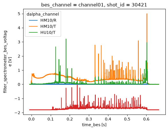
PF Active#
profiles = xr.open_zarr(store, group='pf_active')
fig, axes = plt.subplots(2, 1, figsize=(10, 6))

# coil_current includes the central solenoid (the 'SOL' channel), which
# carries the largest current; the legend identifies each coil channel.
profiles['coil_current'].plot.line(x='time', ax=axes[0])
profiles['coil_voltage'].plot.line(x='time', ax=axes[1])

plt.tight_layout()
profiles
<xarray.Dataset> Size: 2MB
Dimensions:                            (current_channel: 13, time: 15305,
                                        voltage_channel: 5,
                                        p2_inner_lower_coordinate_element: 12,
                                        p2_inner_upper_coordinate_element: 12,
                                        p2_outer_lower_coordinate_element: 8,
                                        p2_outer_upper_coordinate_element: 8,
                                        ...
                                        p4_upper_coordinate_element: 23,
                                        p5_lower_coordinate_element: 23,
                                        p5_upper_coordinate_element: 23,
                                        p6_lower_coordinate_element: 4,
                                        p6_upper_coordinate_element: 4,
                                        sol_coordinate_element: 656)
Coordinates: (12/17)
  * current_channel                    (current_channel) StringDType() 208B '...
  * time                               (time) float64 122kB -0.1 ... 0.6652
  * voltage_channel                    (voltage_channel) StringDType() 80B '/...
  * p2_inner_lower_coordinate_element  (p2_inner_lower_coordinate_element) StringDType() 192B ...
  * p2_inner_upper_coordinate_element  (p2_inner_upper_coordinate_element) StringDType() 192B ...
  * p2_outer_lower_coordinate_element  (p2_outer_lower_coordinate_element) StringDType() 128B ...
    ...                                 ...
  * p5_lower_coordinate_element        (p5_lower_coordinate_element) StringDType() 368B ...
  * p5_upper_coordinate_element        (p5_upper_coordinate_element) StringDType() 368B ...
  * p6_lower_coordinate_element        (p6_lower_coordinate_element) StringDType() 64B ...
  * p6_upper_coordinate_element        (p6_upper_coordinate_element) StringDType() 64B ...
  * sol_coordinate_element             (sol_coordinate_element) StringDType() 10kB ...
    shot_id                            int64 8B 30421
Data variables: (12/54)
    coil_current                       (current_channel, time) float64 2MB ...
    coil_voltage                       (voltage_channel, time) float64 612kB ...
    p2_inner_lower_height              (p2_inner_lower_coordinate_element) float32 48B ...
    p2_inner_lower_r                   (p2_inner_lower_coordinate_element) float32 48B ...
    p2_inner_lower_width               (p2_inner_lower_coordinate_element) float32 48B ...
    p2_inner_lower_z                   (p2_inner_lower_coordinate_element) float32 48B ...
    ...                                 ...
    p6_upper_width                     (p6_upper_coordinate_element) float32 16B ...
    p6_upper_z                         (p6_upper_coordinate_element) float32 16B ...
    sol_height                         (sol_coordinate_element) float32 3kB ...
    sol_r                              (sol_coordinate_element) float32 3kB ...
    sol_width                          (sol_coordinate_element) float32 3kB ...
    sol_z                              (sol_coordinate_element) float32 3kB ...
Attributes:
    name:          pf_active
    description:
    imas:          pf_active
    license_name:  Creative Commons 4.0 BY-SA
    license_url:   https://creativecommons.org/licenses/by-sa/4.0/
    ingested_at:   2026-09-24T17:11:57Z
    commit_url:    https://github.com/ukaea/fair-mast-ingestion/tree/ed6ea4e2...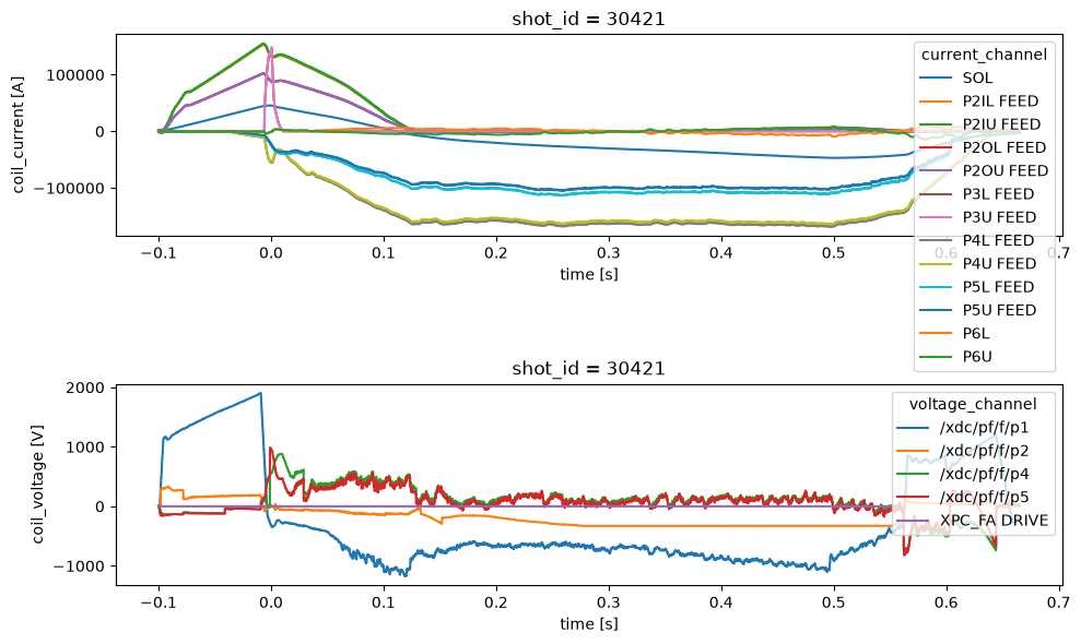
Soft X-rays#
profiles = xr.open_zarr(store, group='soft_x_rays')
fig, axes = plt.subplots(3, 1)


profiles['horizontal_cam_lower'].plot.line(x='time', ax=axes[1], add_legend=False)
axes[1].set_ylim(0, 0.02)

profiles['horizontal_cam_upper'].plot.line(x='time', ax=axes[2], add_legend=False)
axes[2].set_ylim(0, 0.02)

if "tangential_cam" in profiles:
    profiles['tangential_cam'].plot.line(x='time', ax=axes[0], add_legend=False)
    axes[0].set_ylim(0, 0.2)

plt.tight_layout()
profiles
<xarray.Dataset> Size: 168MB
Dimensions:                                (horizontal_cam_lower_channel: 18,
                                            time: 382601,
                                            horizontal_cam_lower_geometry_channel: 18,
                                            horizontal_cam_upper_channel: 18,
                                            horizontal_cam_upper_geometry_channel: 18,
                                            inner_vertical_cam_geometry_channel: 12,
                                            outer_vertical_cam_geometry_channel: 12,
                                            tangential_cam_channel: 18,
                                            tangential_cam_geometry_channel: 18,
                                            third_horizontal_cam_geometry_channel: 18)
Coordinates:
  * horizontal_cam_lower_channel           (horizontal_cam_lower_channel) StringDType() 288B ...
  * time                                   (time) float64 3MB -0.1 ... 0.6652
  * horizontal_cam_lower_geometry_channel  (horizontal_cam_lower_geometry_channel) StringDType() 288B ...
  * horizontal_cam_upper_channel           (horizontal_cam_upper_channel) StringDType() 288B ...
  * horizontal_cam_upper_geometry_channel  (horizontal_cam_upper_geometry_channel) StringDType() 288B ...
  * inner_vertical_cam_geometry_channel    (inner_vertical_cam_geometry_channel) StringDType() 192B ...
  * outer_vertical_cam_geometry_channel    (outer_vertical_cam_geometry_channel) StringDType() 192B ...
  * tangential_cam_channel                 (tangential_cam_channel) StringDType() 288B ...
  * tangential_cam_geometry_channel        (tangential_cam_geometry_channel) StringDType() 288B ...
  * third_horizontal_cam_geometry_channel  (third_horizontal_cam_geometry_channel) StringDType() 288B ...
    shot_id                                int64 8B 30421
Data variables: (12/33)
    horizontal_cam_lower                   (horizontal_cam_lower_channel, time) float64 55MB ...
    horizontal_cam_lower_endpoint_r        (horizontal_cam_lower_geometry_channel) float64 144B ...
    horizontal_cam_lower_endpoint_z        (horizontal_cam_lower_geometry_channel) float64 144B ...
    horizontal_cam_lower_origin_r          (horizontal_cam_lower_geometry_channel) float64 144B ...
    horizontal_cam_lower_origin_z          (horizontal_cam_lower_geometry_channel) float64 144B ...
    horizontal_cam_lower_phi               (horizontal_cam_lower_geometry_channel) float64 144B ...
    ...                                     ...
    tangential_cam_phi                     (tangential_cam_geometry_channel) float64 144B ...
    third_horizontal_cam_endpoint_r        (third_horizontal_cam_geometry_channel) float64 144B ...
    third_horizontal_cam_endpoint_z        (third_horizontal_cam_geometry_channel) float64 144B ...
    third_horizontal_cam_origin_r          (third_horizontal_cam_geometry_channel) float64 144B ...
    third_horizontal_cam_origin_z          (third_horizontal_cam_geometry_channel) float64 144B ...
    third_horizontal_cam_phi               (third_horizontal_cam_geometry_channel) float64 144B ...
Attributes:
    name:          soft_x_rays
    description:   Soft X-rays tomography diagnostic
    imas:          soft_x_rays
    license_name:  Creative Commons 4.0 BY-SA
    license_url:   https://creativecommons.org/licenses/by-sa/4.0/
    ingested_at:   2026-09-24T17:21:02Z
    commit_url:    https://github.com/ukaea/fair-mast-ingestion/tree/ed6ea4e2...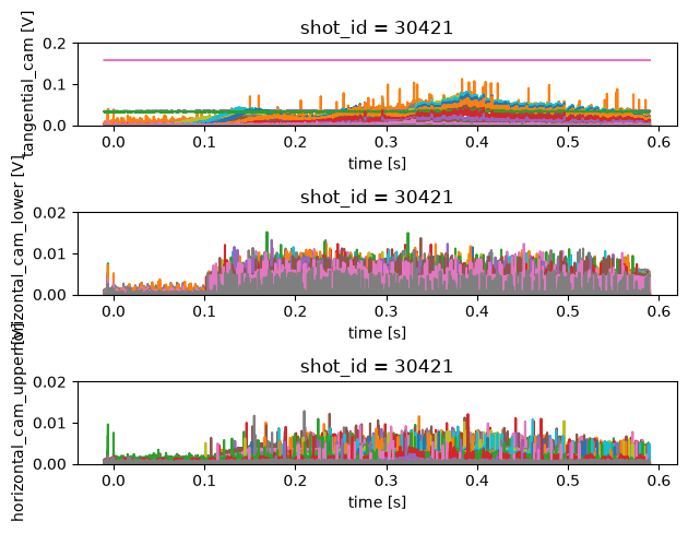
Thomson Profiles#
Thomson scattering measurements in a tokamak provide information about the plasma’s electron temperature and density profiles. The diagnostic analyses the scattering of laser light off free electrons in the plasma from a number of radial channels.
Below we plot the following profiles measured by the Thomson diagnostic
\(T_e\) - Electron temperature
\(N_e\) - Electron density
\(P_e\) - Electron pressure
profiles = xr.open_zarr(store, group='thomson_scattering')
profiles

fig, axes = plt.subplots(3, 1)
axes = axes.flatten()
profiles.t_e.plot(x='time', y='major_radius', ax=axes[0])
profiles.n_e.plot(x='time', y='major_radius', ax=axes[1])
profiles.p_e.plot(x='time', y='major_radius', ax=axes[2])
plt.tight_layout()

profiles
<xarray.Dataset> Size: 819kB
Dimensions:       (major_radius: 120, time: 283)
Coordinates:
  * major_radius  (major_radius) float64 960B 0.3 0.31 0.32 ... 1.47 1.48 1.49
  * time          (time) float32 1kB 0.004166 0.008332 ... 0.6042 0.6042
    shot_id       int64 8B ...
Data variables:
    n_e           (major_radius, time) float64 272kB ...
    n_e_core      (time) float32 1kB ...
    p_e           (major_radius, time) float64 272kB ...
    t_e           (major_radius, time) float64 272kB ...
    t_e_core      (time) float32 1kB ...
Attributes:
    name:          thomson_scattering
    description:   Thomson scattering diagnostic
    imas:          thomson_scattering
    license_name:  Creative Commons 4.0 BY-SA
    license_url:   https://creativecommons.org/licenses/by-sa/4.0/
    ingested_at:   2026-09-24T17:19:31Z
    commit_url:    https://github.com/ukaea/fair-mast-ingestion/tree/ed6ea4e2...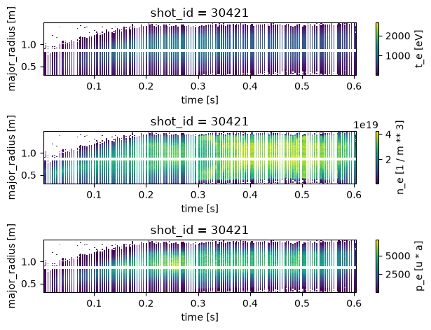
fig, axes = plt.subplots(2, 1)
profiles['t_e_core'].plot(x='time', ax=axes[0])
profiles['n_e_core'].plot(x='time', ax=axes[1])
for ax in axes:
    ax.grid('on', alpha=0.5)
plt.tight_layout()
profiles
<xarray.Dataset> Size: 819kB
Dimensions:       (major_radius: 120, time: 283)
Coordinates:
  * major_radius  (major_radius) float64 960B 0.3 0.31 0.32 ... 1.47 1.48 1.49
  * time          (time) float32 1kB 0.004166 0.008332 ... 0.6042 0.6042
    shot_id       int64 8B ...
Data variables:
    n_e           (major_radius, time) float64 272kB ...
    n_e_core      (time) float32 1kB ...
    p_e           (major_radius, time) float64 272kB ...
    t_e           (major_radius, time) float64 272kB ...
    t_e_core      (time) float32 1kB ...
Attributes:
    name:          thomson_scattering
    description:   Thomson scattering diagnostic
    imas:          thomson_scattering
    license_name:  Creative Commons 4.0 BY-SA
    license_url:   https://creativecommons.org/licenses/by-sa/4.0/
    ingested_at:   2026-09-24T17:19:31Z
    commit_url:    https://github.com/ukaea/fair-mast-ingestion/tree/ed6ea4e2...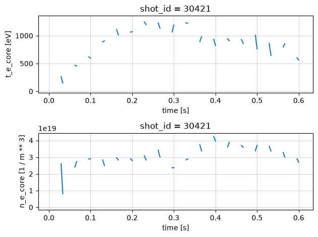
CXRS Profiles#
Charge Exchange Recombination Spectroscopy (CXRS) measurements provide information about ion temperature and plasma rotation. This diagnostic analyses the light emitted from charge exchange reactions between injected neutral beams and plasma ions.
Below we plot the following profiles measured by the CXRS diagnostic
\(T_i\) - Ion temperature
\(V_i\) - Ion velocity
profiles = xr.open_zarr(store, group='charge_exchange')

fig, axes = plt.subplots(2, 1)
for name, ax in [('t_i', axes[0]), ('v_i', axes[1])]:
    da = profiles[name]
    da.plot(x='time', y='major_radius', ax=ax, vmax=1000)
    # clip the axes to the region where the diagnostic actually has data
    valid = da.notnull()
    times = da['time'].where(valid.any('major_radius'), drop=True)
    radii = da['major_radius'].where(valid.any('time'), drop=True)
    ax.set_xlim(float(times.min()), float(times.max()))
    ax.set_ylim(float(radii.min()), float(radii.max()))

plt.tight_layout()
profiles
<xarray.Dataset> Size: 402kB
Dimensions:       (major_radius: 161, time: 155)
Coordinates:
  * major_radius  (major_radius) float64 1kB 0.0 0.01 0.02 ... 1.58 1.59 1.6
  * time          (time) float64 1kB -0.1 -0.095 -0.09 ... 0.66 0.665 0.67
    shot_id       int64 8B ...
Data variables:
    t_i           (major_radius, time) float64 200kB nan nan nan ... nan nan nan
    v_i           (major_radius, time) float64 200kB nan nan nan ... nan nan nan
Attributes:
    name:          charge_exchange
    description:
    imas:          charge_exchange
    license_name:  Creative Commons 4.0 BY-SA
    license_url:   https://creativecommons.org/licenses/by-sa/4.0/
    ingested_at:   2026-09-24T17:19:31Z
    commit_url:    https://github.com/ukaea/fair-mast-ingestion/tree/ed6ea4e2...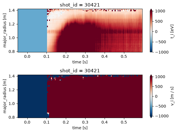
Equilibrium#
profiles = xr.open_zarr(store, group='equilibrium')

profile_1d = profiles[["beta_tor_normal", "wmhd", "li", "elongation", "triangularity_upper", "q95", "vloop_dynamic", "ip_rating", "lcfs_r", "lcfs_z"]]
plot_1d_profiles(profile_1d)

profiles
<xarray.Dataset> Size: 13MB
Dimensions:                          (time: 155, psi_norm: 65,
                                      n_b_field_pol_probe: 78, n_flux_loop: 46,
                                      z: 65, major_radius: 65,
                                      n_boundary_coords: 139,
                                      n_pf_current: 101, profile_r: 65,
                                      n_x_points_r: 2, n_x_points_z: 2)
Coordinates:
  * time                             (time) float64 1kB -0.1 -0.095 ... 0.67
  * psi_norm                         (psi_norm) float32 260B 0.0 0.01562 ... 1.0
  * n_b_field_pol_probe              (n_b_field_pol_probe) float32 312B 0.0 ....
  * n_flux_loop                      (n_flux_loop) float32 184B 0.0 1.0 ... 45.0
  * z                                (z) float32 260B -2.0 -1.938 ... 1.938 2.0
  * major_radius                     (major_radius) float64 520B 0.06 ... 1.98
  * n_boundary_coords                (n_boundary_coords) float32 556B 0.0 ......
  * n_pf_current                     (n_pf_current) float32 404B 0.0 ... 100.0
  * profile_r                        (profile_r) float32 260B 0.0 ... 1.0
  * n_x_points_r                     (n_x_points_r) StringDType() 32B 'XPOINT...
  * n_x_points_z                     (n_x_points_z) StringDType() 32B 'XPOINT...
    shot_id                          int64 8B ...
Data variables: (12/77)
    area                             (time) float64 1kB ...
    area_psi                         (psi_norm, time) float64 81kB ...
    b_field_pol_probe_ang            (n_b_field_pol_probe) float32 312B ...
    b_field_pol_probe_chi_squared    (time, n_b_field_pol_probe) float64 97kB ...
    b_field_pol_probe_len            (n_b_field_pol_probe) float32 312B ...
    b_field_pol_probe_measured       (time, n_b_field_pol_probe) float64 97kB ...
    ...                               ...
    vloop_static                     (time) float64 1kB ...
    volume                           (time) float64 1kB ...
    volume_psi                       (psi_norm, time) float64 81kB ...
    wmhd                             (time) float64 1kB ...
    x_point_r                        (n_x_points_r, time) float64 2kB ...
    x_point_z                        (n_x_points_z, time) float64 2kB ...
Attributes:
    name:          equilibrium
    description:   Description of a 2D, axi-symmetric, tokamak equilibrium; r...
    imas:          equilibrium
    license_name:  Creative Commons 4.0 BY-SA
    license_url:   https://creativecommons.org/licenses/by-sa/4.0/
    ingested_at:   2026-09-24T17:10:47Z
    commit_url:    https://github.com/ukaea/fair-mast-ingestion/tree/ed6ea4e2...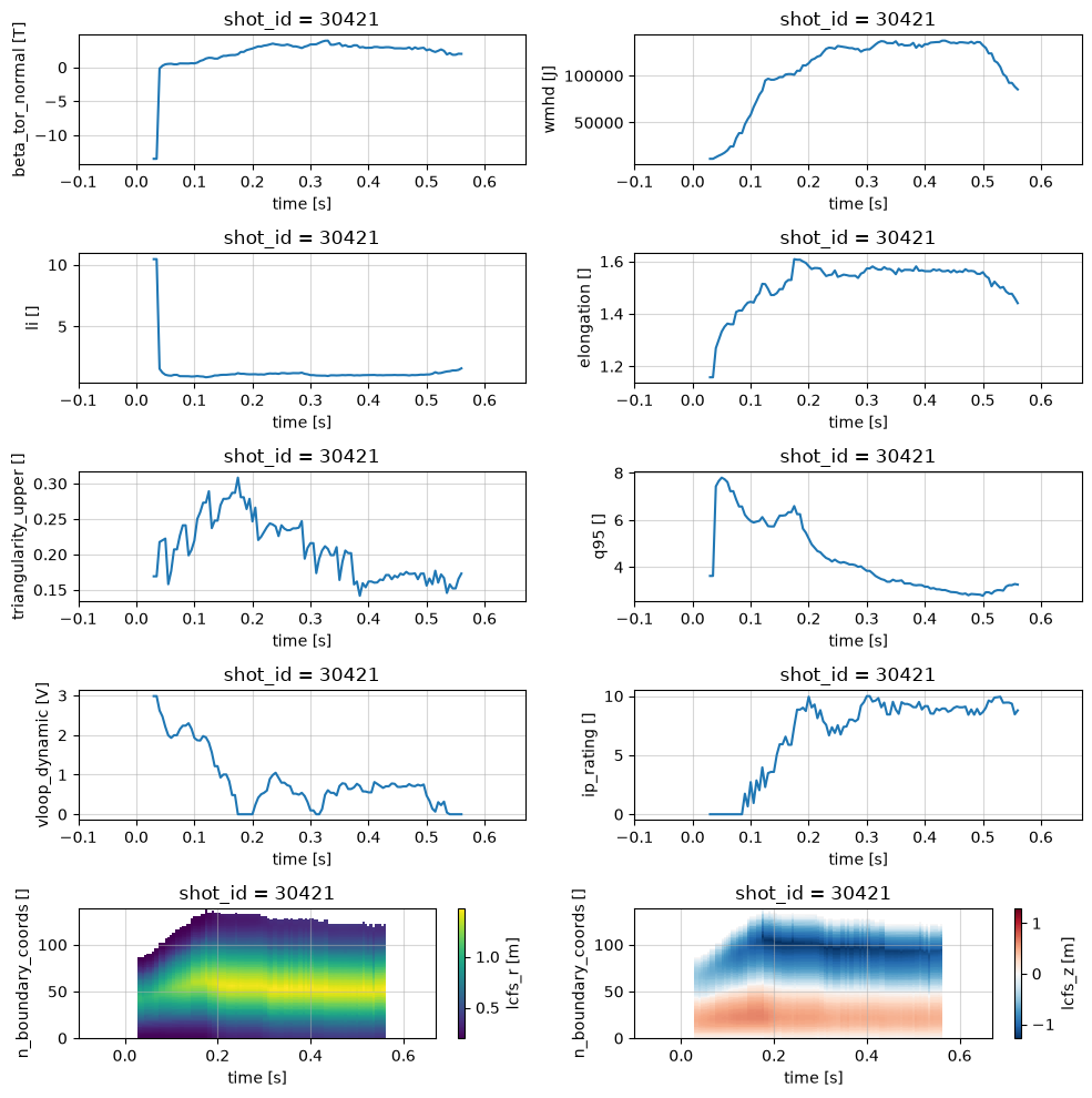
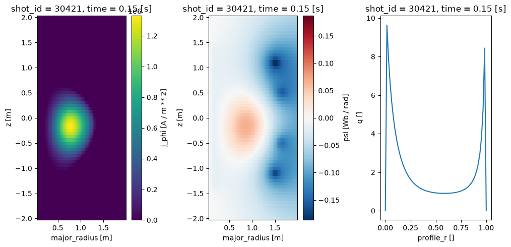
fig, axes = plt.subplots(1, 3, figsize=(10, 5))

profiles['j_phi'].isel(time=50).plot(ax=axes[0], x='major_radius')
profiles['psi'].isel(time=50).plot(ax=axes[1], x='major_radius')
profiles['q'].isel(time=50).plot(ax=axes[2])
plt.tight_layout()
EFIT constraint axes#
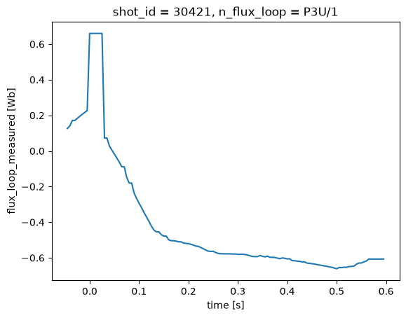
EFIT’s flux loop and magnetic probe constraints are stored on numbered axes, n_flux_loop (46 loops) and n_b_field_pol_probe (78 probes), in EFIT’s detector order. Each constraint variable carries the detector names for its axis in an attribute, n_flux_loop_order or n_b_field_pol_probe_order, stored as a JSON list.
Use it to select a detector by name:
import json

eq = xr.open_zarr(store, group='equilibrium')
loops = json.loads(eq.flux_loop_measured.attrs['n_flux_loop_order'])

eq.flux_loop_measured.isel(n_flux_loop=loops.index('P3U/1'))
<xarray.DataArray 'flux_loop_measured' (time: 155)> Size: 1kB
[155 values with dtype=float64]
Coordinates:
  * time         (time) float64 1kB -0.1 -0.095 -0.09 -0.085 ... 0.66 0.665 0.67
    n_flux_loop  float32 4B 14.0
    shot_id      int64 8B ...
Attributes:
    imas:               equilibrium.time_slice[:].constraints.flux_loop[:].me...
    description:        Measured flux loop value used as a constraint in the ...
    name:               flux_loop_measured
    uda_name:           EFM_SILOP_(X)
    n_flux_loop_order:  ["CC01", "CC02", "CC03", "CC04", "CC05", "CC06", "CC0...
units: WbOr put the names on the axis, so you can use .sel() throughout. The probes work the same way with n_b_field_pol_probe and n_b_field_pol_probe_order.
probes = json.loads(eq.b_field_pol_probe_measured.attrs['n_b_field_pol_probe_order'])
eq_named = eq.assign_coords(n_flux_loop=loops, n_b_field_pol_probe=probes)

eq_named.flux_loop_measured.sel(n_flux_loop='P3U/1').plot()
plt.show()
Only some detectors were digitised: 15 of the 46 flux loops and 58 of the 78 probes. flux_loop_weight is zero for every loop on MAST, so use the measured values to find them. b_field_pol_probe_weight does show which probes the fit used.
# Non-zero at any time (max ignores the NaNs outside the fit window)
loop_digitised = abs(eq_named.flux_loop_measured).max('time') > 0
probe_digitised = abs(eq_named.b_field_pol_probe_measured).max('time') > 0
probe_used = abs(eq_named.b_field_pol_probe_weight).max('time') > 0

print(f'{int(loop_digitised.sum())} of {len(loops)} flux loops digitised')
print(f'{int(probe_digitised.sum())} of {len(probes)} probes digitised, {int(probe_used.sum())} used by the fit')
print('Digitised loops:', eq_named.n_flux_loop[loop_digitised].values.tolist())
15 of 46 flux loops digitised
58 of 78 probes digitised, 35 used by the fit
Digitised loops: ['CC03', 'CC04', 'CC05', 'CC07', 'CC09', 'P3U/1', 'P3U/4', 'P4U/4', 'P5U/1', 'P3L/4', 'P4L/1', 'P4L/4', 'P5L/1', 'P5L/4', 'P6L/1']
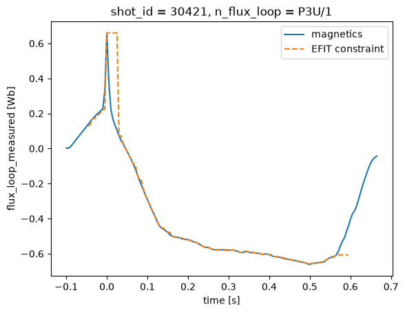
To compare EFIT’s constraints with the measurements in magnetics, match loops by name, not by index: magnetics.flux_loop_flux holds only the 15 digitised loops, in a different order, on a finer time grid.
mag = xr.open_zarr(store, group='magnetics')
names = [str(name) for name in mag.flux_loop_channel.values]

efit = eq_named.flux_loop_measured.sel(n_flux_loop=names)
measured = mag.flux_loop_flux.interp(time=eq.time)

fig, ax = plt.subplots()
measured.sel(flux_loop_channel='P3U/1').plot(ax=ax, label='magnetics')
efit.sel(n_flux_loop='P3U/1').plot(ax=ax, label='EFIT constraint', linestyle='--')
ax.legend()
plt.show()
Gas Injection#
profiles = xr.open_zarr(store, group='gas_injection')

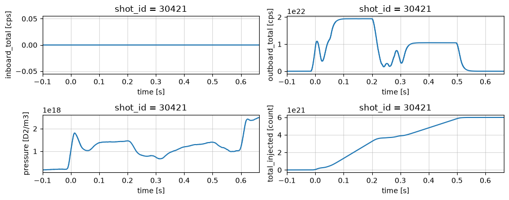
plot_1d_profiles(profiles[["inboard_total", "outboard_total", "pressure", "total_injected"]])
plt.tight_layout()
profiles
<xarray.Dataset> Size: 5MB
Dimensions:               (time: 15305, target_valve_channel: 12,
                           valve_channel: 20)
Coordinates:
  * time                  (time) float64 122kB -0.1 -0.09995 ... 0.6652 0.6652
  * target_valve_channel  (target_valve_channel) StringDType() 192B 'g1' ... ...
  * valve_channel         (valve_channel) StringDType() 320B 'tc5a' ... 'ibflb'
    shot_id               int64 8B ...
Data variables:
    inboard_total         (time) float64 122kB ...
    outboard_total        (time) float64 122kB ...
    pressure              (time) float64 122kB ...
    total_injected        (time) float64 122kB ...
    valve_target_voltage  (target_valve_channel, time) float64 1MB ...
    valve_voltage         (valve_channel, time) float64 2MB ...
Attributes:
    name:          gas_injection
    description:   Gas injection by a system of pipes and valves.
    imas:          gas_injection
    license_name:  Creative Commons 4.0 BY-SA
    license_url:   https://creativecommons.org/licenses/by-sa/4.0/
    ingested_at:   2026-09-24T17:11:01Z
    commit_url:    https://github.com/ukaea/fair-mast-ingestion/tree/ed6ea4e2...