! pip install matplotlib pandas seaborn intake intake_parquet
Show code cell output
Requirement already satisfied: matplotlib in /Users/rt2549/miniconda3/envs/mast/lib/python3.11/site-packages (3.9.0)
Requirement already satisfied: pandas in /Users/rt2549/miniconda3/envs/mast/lib/python3.11/site-packages (2.0.3)
Collecting seaborn
  Using cached seaborn-0.13.2-py3-none-any.whl.metadata (5.4 kB)
Requirement already satisfied: intake in /Users/rt2549/miniconda3/envs/mast/lib/python3.11/site-packages (2.0.5)
Collecting intake_parquet
  Using cached intake_parquet-0.3.0-py3-none-any.whl.metadata (1.8 kB)
Requirement already satisfied: contourpy>=1.0.1 in /Users/rt2549/miniconda3/envs/mast/lib/python3.11/site-packages (from matplotlib) (1.2.1)
Requirement already satisfied: cycler>=0.10 in /Users/rt2549/miniconda3/envs/mast/lib/python3.11/site-packages (from matplotlib) (0.12.1)
Requirement already satisfied: fonttools>=4.22.0 in /Users/rt2549/miniconda3/envs/mast/lib/python3.11/site-packages (from matplotlib) (4.53.0)
Requirement already satisfied: kiwisolver>=1.3.1 in /Users/rt2549/miniconda3/envs/mast/lib/python3.11/site-packages (from matplotlib) (1.4.5)
Requirement already satisfied: numpy>=1.23 in /Users/rt2549/miniconda3/envs/mast/lib/python3.11/site-packages (from matplotlib) (1.25.2)
Requirement already satisfied: packaging>=20.0 in /Users/rt2549/miniconda3/envs/mast/lib/python3.11/site-packages (from matplotlib) (24.0)
Requirement already satisfied: pillow>=8 in /Users/rt2549/miniconda3/envs/mast/lib/python3.11/site-packages (from matplotlib) (10.3.0)
Requirement already satisfied: pyparsing>=2.3.1 in /Users/rt2549/miniconda3/envs/mast/lib/python3.11/site-packages (from matplotlib) (3.1.2)
Requirement already satisfied: python-dateutil>=2.7 in /Users/rt2549/miniconda3/envs/mast/lib/python3.11/site-packages (from matplotlib) (2.9.0.post0)
Requirement already satisfied: pytz>=2020.1 in /Users/rt2549/miniconda3/envs/mast/lib/python3.11/site-packages (from pandas) (2024.1)
Requirement already satisfied: tzdata>=2022.1 in /Users/rt2549/miniconda3/envs/mast/lib/python3.11/site-packages (from pandas) (2024.1)
Requirement already satisfied: fsspec>=2023.0.0 in /Users/rt2549/miniconda3/envs/mast/lib/python3.11/site-packages (from intake) (2024.5.0)
Requirement already satisfied: pyyaml in /Users/rt2549/miniconda3/envs/mast/lib/python3.11/site-packages (from intake) (6.0.1)
Requirement already satisfied: appdirs in /Users/rt2549/miniconda3/envs/mast/lib/python3.11/site-packages (from intake) (1.4.4)
Collecting fastparquet (from intake_parquet)
  Downloading fastparquet-2024.11.0-cp311-cp311-macosx_11_0_arm64.whl.metadata (4.2 kB)
Requirement already satisfied: pyarrow in /Users/rt2549/miniconda3/envs/mast/lib/python3.11/site-packages (from intake_parquet) (12.0.1)
Requirement already satisfied: six>=1.5 in /Users/rt2549/miniconda3/envs/mast/lib/python3.11/site-packages (from python-dateutil>=2.7->matplotlib) (1.16.0)
Collecting cramjam>=2.3 (from fastparquet->intake_parquet)
  Downloading cramjam-2.9.0-cp311-cp311-macosx_11_0_arm64.whl.metadata (4.9 kB)
Using cached seaborn-0.13.2-py3-none-any.whl (294 kB)
Using cached intake_parquet-0.3.0-py3-none-any.whl (5.4 kB)
Downloading fastparquet-2024.11.0-cp311-cp311-macosx_11_0_arm64.whl (683 kB)
?25l   ━━━━━━━━━━━━━━━━━━━━━━━━━━━━━━━━━━━━━━━━ 0.0/683.8 kB ? eta -:--:--
━━━━━━━━━━━╸━━━━━━━━━━━━━━━━━━━━━━━━━━━━ 204.8/683.8 kB 5.3 MB/s eta 0:00:01
   ━━━━━━━━━━━━━━━━━━━━━━━━━━━━━━╸━━━━━━━━━ 522.2/683.8 kB 6.9 MB/s eta 0:00:01
   ━━━━━━━━━━━━━━━━━━━━━━━━━━━━━━━━━━━━━━╸━ 665.6/683.8 kB 5.8 MB/s eta 0:00:01
   ━━━━━━━━━━━━━━━━━━━━━━━━━━━━━━━━━━━━━━━━ 683.8/683.8 kB 5.3 MB/s eta 0:00:00
?25hDownloading cramjam-2.9.0-cp311-cp311-macosx_11_0_arm64.whl (1.9 MB)
?25l   ━━━━━━━━━━━━━━━━━━━━━━━━━━━━━━━━━━━━━━━━ 0.0/1.9 MB ? eta -:--:--
   ━━━━━━╺━━━━━━━━━━━━━━━━━━━━━━━━━━━━━━━━━ 0.3/1.9 MB 8.4 MB/s eta 0:00:01
   ━━━━━━━━━━━━╺━━━━━━━━━━━━━━━━━━━━━━━━━━━ 0.6/1.9 MB 8.3 MB/s eta 0:00:01
━━━━━━━━━━━━━━━━━━╸━━━━━━━━━━━━━━━━━━━━━ 0.9/1.9 MB 8.2 MB/s eta 0:00:01
━━━━━━━━━━━━━━━━━━━━━━━━━╸━━━━━━━━━━━━━━ 1.2/1.9 MB 8.2 MB/s eta 0:00:01
   ━━━━━━━━━━━━━━━━━━━━━━━━━━━━━━━╸━━━━━━━━ 1.5/1.9 MB 8.2 MB/s eta 0:00:01
   ━━━━━━━━━━━━━━━━━━━━━━━━━━━━━━━━━━━━━━╸━ 1.9/1.9 MB 8.1 MB/s eta 0:00:01
   ━━━━━━━━━━━━━━━━━━━━━━━━━━━━━━━━━━━━━━━━ 1.9/1.9 MB 7.6 MB/s eta 0:00:00
?25h
Installing collected packages: cramjam, seaborn, fastparquet, intake_parquet
Successfully installed cramjam-2.9.0 fastparquet-2024.11.0 intake_parquet-0.3.0 seaborn-0.13.2
import pandas as pd
import seaborn as sns
import intake
import matplotlib.pyplot as plt

plt.rcParams["font.family"] = "sans"
plt.rcParams["font.size"] = 8
sns.set_palette('muted')
Tutorial: Exploring Shot Metadata#
This notebook contains a demonstration of plotting several of the summary statistics that accompany the shot metadata.
Firstly, we’re going to load all the shot data into a pandas dataframe:
catalog  = intake.open_catalog(f'https://mastapp.site/intake/catalog.yml')
summary = pd.DataFrame(catalog.index.level1.shots().read())
# summary = df.loc[df.campaign == 'M9']
summary
| url | preshot_description | postshot_description | campaign | current_range | divertor_config | plasma_shape | comissioner | facility | shot_id | ... | cpf_vol_ipmax | cpf_vol_max | cpf_vol_truby | cpf_wmhd_ipmax | cpf_wmhd_max | cpf_wmhd_truby | cpf_zeff_ipmax | cpf_zeff_max | cpf_zeff_truby | cpf_zmag_efit | |
|---|---|---|---|---|---|---|---|---|---|---|---|---|---|---|---|---|---|---|---|---|---|
| 0 | s3://mast/level1/shots/11695.zarr | \n0.1T TF SHOT\n | \nOK\n | M5 | None | Conventional | None | None | MAST | 11695 | ... | NaN | NaN | NaN | NaN | NaN | NaN | NaN | NaN | NaN | NaN |
| 1 | s3://mast/level1/shots/11696.zarr | \nSTANDARD 0.3T TF SHOT\n | \nOK\n | M5 | None | Conventional | None | None | MAST | 11696 | ... | NaN | NaN | NaN | NaN | NaN | NaN | NaN | NaN | NaN | NaN |
| 2 | s3://mast/level1/shots/11697.zarr | \nRAISE TO 0.5T\n | \nOK, ALARMS ARE LOWER\n | M5 | None | Conventional | None | None | MAST | 11697 | ... | NaN | NaN | NaN | NaN | NaN | NaN | NaN | NaN | NaN | NaN |
| 3 | s3://mast/level1/shots/11698.zarr | \nRAISE TO .56T\n | \nSTILL ALARMS BUT LOWER AGAIN\n | M5 | None | Conventional | None | None | MAST | 11698 | ... | NaN | NaN | NaN | NaN | NaN | NaN | NaN | NaN | NaN | NaN |
| 4 | s3://mast/level1/shots/11699.zarr | \nRAISE TO .58T\n | \nOK\n | M5 | None | Conventional | None | None | MAST | 11699 | ... | NaN | NaN | NaN | NaN | NaN | NaN | NaN | NaN | NaN | NaN |
| ... | ... | ... | ... | ... | ... | ... | ... | ... | ... | ... | ... | ... | ... | ... | ... | ... | ... | ... | ... | ... | ... |
| 15916 | s3://mast/level1/shots/30467.zarr | \nRepeat with new neutron camera position.\ncH... | \nTwo times lower DD neutron rate than referen... | M9 | 700 kA | Conventional | Connected Double Null | None | MAST | 30467 | ... | 9.029202 | 9.046394 | 0.0 | 49469.122469 | 52653.445 | 0.0 | NaN | NaN | NaN | 0.013202 |
| 15917 | s3://mast/level1/shots/30468.zarr | \nRepeat with new neutron camera position.\ncH... | \nGood beam.\nGood repeat.\n | M9 | 700 kA | Conventional | Lower Single Null | None | MAST | 30468 | ... | 9.102411 | 9.107017 | 0.0 | 48516.962675 | 49382.133 | 0.0 | NaN | NaN | NaN | 0.012445 |
| 15918 | s3://mast/level1/shots/30469.zarr | \nRepeat with increased beam power (74 kV)\ncH... | \nGood shot. Modes present.\n | M9 | 700 kA | Conventional | Connected Double Null | None | MAST | 30469 | ... | 8.988730 | 9.047923 | 0.0 | 47466.249616 | 49115.805 | 0.0 | NaN | NaN | NaN | 0.015299 |
| 15919 | s3://mast/level1/shots/30470.zarr | \nRepeat last using hydrogen in outboard and c... | \nNo HF gas.\n | M9 | 700 kA | Conventional | None | None | MAST | 30470 | ... | 9.687049 | 10.055509 | 0.0 | 17290.432865 | 22310.516 | 0.0 | NaN | NaN | NaN | 0.015164 |
| 15920 | s3://mast/level1/shots/30471.zarr | \nThe last plasma:\nConvert to i/b Helios 1724... | \nGood shot.\n | M9 | 700 kA | Conventional | Lower Single Null | None | MAST | 30471 | ... | 8.817559 | 9.283702 | 0.0 | 38063.582380 | 40906.090 | 0.0 | NaN | NaN | NaN | 0.014340 |
15921 rows × 283 columns
Summary Statistics About Shots#
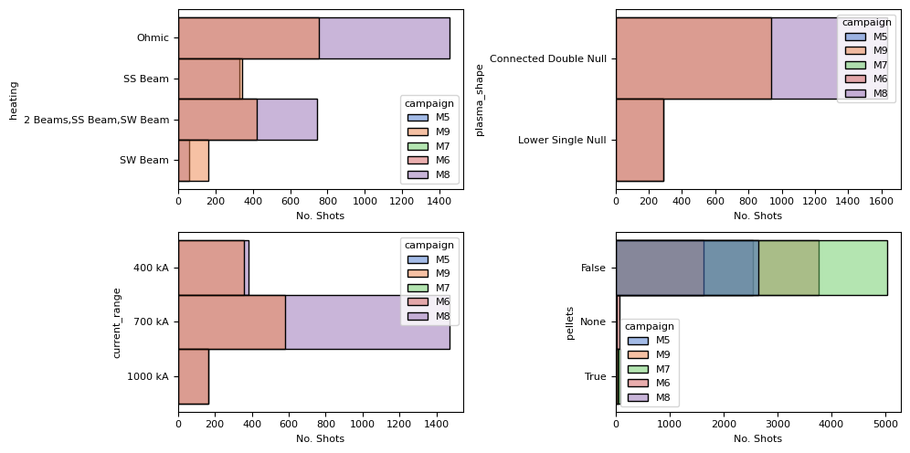
Let’s look at a summary of simple counts of different shot metadata.
fig, axes = plt.subplots(2, 2, figsize=(10, 5))
ax1, ax2, ax3, ax4 = axes.flatten()

sns.histplot(summary, y='heating', hue='campaign', ax=ax1)
sns.histplot(summary, y='plasma_shape', hue='campaign', ax=ax2)
sns.histplot(summary, y='current_range', hue='campaign', ax=ax3)
sns.histplot(summary, y=summary.pellets.astype(str), hue='campaign', ax=ax4)

for ax in axes.flatten():
    ax.set_xlabel('No. Shots')

plt.tight_layout()
Plasma Beta (
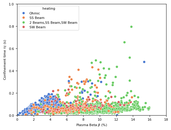
This plot can show how the efficiency of energy confinement varies with plasma pressure.
plt.figure()
sns.scatterplot(summary, y='cpf_tautot_max', x='cpf_betmhd_max', hue='heating')
plt.xlim(0, 18)
plt.ylim(0, 1)
# plt.yscale('log')
plt.ylabel('Confinement time $\\tau_E$ (s)')
plt.xlabel('Plasma Beta $\\beta$ (%)')
Text(0.5, 0, 'Plasma Beta $\\beta$ (%)')
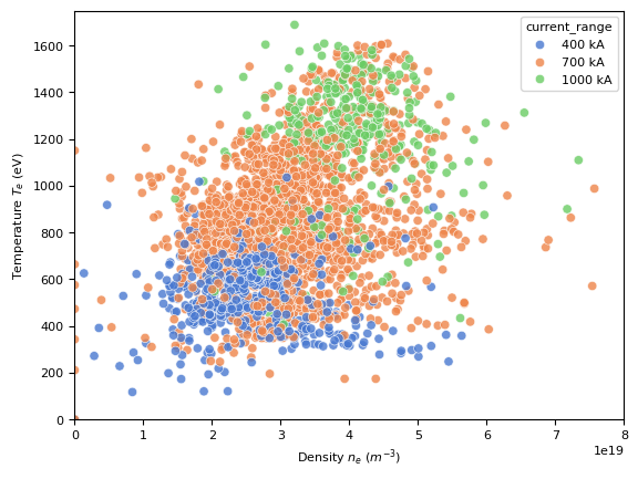
Plasma Temperature (
This can reveal the relationship between temperature and density, which is critical for achieving the conditions necessary for fusion.
plt.figure()
sns.scatterplot(summary, y='cpf_te0_ipmax', x='cpf_ne0_ipmax', hue='current_range', alpha=0.8)
plt.xlim(0, .8e20)
plt.ylim(0, 1750)
plt.ylabel('Temperature $T_e$ (eV)')
plt.xlabel('Density $n_e$ ($m^{-3}$)')
Text(0.5, 0, 'Density $n_e$ ($m^{-3}$)')
Plasma Current (
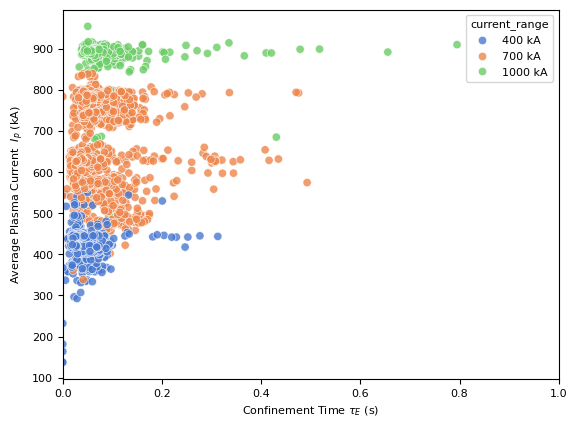
This can indicate how the plasma current affects the confinement time, providing insights into stability and performance.
plt.figure()
sns.scatterplot(summary, y='cpf_ip_av', x='cpf_tautot_max', hue='current_range', alpha=0.8)
plt.xlim(0, 1)
plt.xlabel('Confinement Time $\\tau_E$ (s)')
plt.ylabel('Average Plasma Current  $I_p$ (kA)')
Text(0, 0.5, 'Average Plasma Current $I_p$ (kA)')
