Plasma physics

Introduction

By default, the plasma is assumed to have an up-down asymmetric, single null configuration (although this can be changed with user inputs). A great number of physics models are coded within PROCESS to describe the behaviour of the plasma parameters such as its current, temperature, density, pressure, confinement etc., and also the various limits that define the stable operating domain.

More detail is given in ¹⁸, but this webpage is more up to date.

Plasma Geometry

The plasma geometric major radius $R_0$ (rmajor) and aspect ratio $A$ (aspect) define the size of the plasma torus. The plasma minor radius $a$ (rminor) is calculated from these values. The shape of the plasma cross-section is given by the elongation of the last closed flux surface (LCFS) $\kappa$ (kappa) and the triangularity of the LCFS $\delta$ (triang), which can be scaled automatically with the aspect ratio if required using switch ishape:

• ishape = 0 -- kappa and triang must be input. The elongation and triangularity of the 95% flux surface are calculated as follows ⁸: $$ \kappa_{95} = \kappa / 1.12 $$ $$ \delta_{95} = \delta / 1.5 $$

• ishape = 1 -- kappa and triang must not be input. They are calculated by the following equations, which estimate the largest elongation and triangularity achievable for low aspect ratio machines ($\epsilon = 1/A$) ¹:

$$ \kappa = 2.05 \, (1 + 0.44 \, \epsilon^{2.1}) $$

$$ \delta = 0.53 \, (1 + 0.77 \, \epsilon^3) $$

The values for the plasma shaping parameters at the 95% flux surface are calculated using a fit to a family of equilibria calculated using the FIESTA code, equivalent to ishape = 8.

• ishape = 2 -- the Zohm ITER scaling ² is used to calculate the elongation:

$$ \kappa = F_{kz} \, \times \, \mathrm{minimum} \left( 2.0, \, \, 1.5 + \frac{0.5}{A-1} \right) $$

where input variable fkzohm $= F_{kz}$ may be used to adjust the scaling, while the input value of the triangularity is used unchanged.

• ishape = 3 -- the Zohm ITER scaling is used to calculate the elongation (as for ishape = 2 above), but the triangularity at the 95% flux surface is input via variable triang95, and the LCFS triangularity triang is calculated from it, rather than the other way round.

• ishape = 4 -- the 95% flux surface values kappa95 and triang95 are both used as inputs, and the LCFS values are calculated from them by inverting the equations given above for ishape = 0.

• ishape = 5 -- the 95% flux surface values kappa95 and triang95 are both used as inputs and the LCFS values are calculated from a fit to MAST data:

$$ \kappa = 0.91 \, \kappa_{95} + 0.39 $$

$$ \delta = 0.77 \, \delta_{95} + 0.19 $$

• ishape = 6 -- the input values for kappa and triang are used directly and the 95% flux surface values are calculated using the MAST scaling from ishape = 5.

• ishape = 7 -- the 95% flux surface values kappa95 and triang95 are both used as inputs and the LCFS values are calculated from a fit to FIESTA runs:

$$ \kappa = 0.91 \, \kappa_{95} + 0.39 $$

$$ \delta = 1.38 \, \delta_{95} + 0.05 $$

• ishape = 8 -- the input values for kappa and triang are used directly and the 95% flux surface values are calculated using the FIESTA fit from ishape = 7.

An explicit constraint relating to the plasma's vertical stability may be turned on if required. In principle, the inner surface of the outboard shield could be used as the location of a conducting shell to mitigate the vertical displacement growth rate of plasmas with significant elongation ⁴. The maximum permissible distance $r_{\text{shell, max}}$ of this shell from the geometric centre of the plasma may be set using input parameter cwrmax, such that $r_{\text{shell, max}} =$ cwrmax*rminor. Constraint equation no. 23 should be turned on with iteration variable no. 104 (fcwr) to enforce this.

The plasma surface area, cross-sectional area and volume are calculated using formulations that approximate the LCFS as a revolution of two arcs which intersect the plasma X-points and the plasma midplane outer and inner radii. (This is a reasonable assumption for double-null diverted plasmas, but will be inaccurate for single-null plasmas, snull = 1).

Fusion Reactions

The most likely fusion reaction to be utilised in a power plant is the deuterium-tritium reaction:

$$\mathrm{D + T} \Longrightarrow \mathrm{^{4}He + n + 17.6 \,MeV}$$

20% of the energy produced is given to the alpha particles ($^4$He). The remaining 80% is carried away by the neutrons, which deposit their energy within the blanket and shield and other reactor components. The fraction of the alpha energy deposited in the plasma is falpha.

PROCESS can also model D-$^3$He power plants, which utilise the following primary fusion reaction:

$$\mathrm{D + \text{$^3$He}} \Longrightarrow \mathrm{^{4}He + p + 18.3 \,MeV}$$

The fusion reaction rate is significantly different to that for D-T fusion, and the power flow from the plasma is modified since charged particles are produced rather than neutrons. Because only charged particles (which remain in the plasma) are produced by this reaction, the whole of the fusion power is used to heat the plasma. Useful energy is extracted from the plasma since the radiation power produced is very high, and this, in theory, can be converted to electricity without using a thermal cycle.

Since the temperature required to ignite the D-$^3$He reaction is considerably higher than that for D-T, it is necessary to take into account the following D-D reactions, which have significant reaction rates at such temperatures:

$$\begin{aligned} \mathrm{D + D} & \Longrightarrow \mathrm{^{3}He + n + 3.27 \,MeV} \\ \mathrm{D + D} & \Longrightarrow \mathrm{T + p + 4.03 \,MeV} \end{aligned}$$

Also, as tritium is produced by the latter reaction, D-T fusion also occurs. As a result, there is still a small amount of neutron power extracted from the plasma.

Pure D-$^3$He tokamak power plants do not include breeding blankets, because no tritium needs to be produced for fuel.

The contributions from all four of the above fusion reactions are included in the total fusion power production calculation. The fusion reaction rates are calculated using the parameterizations in ⁴, integrated over the plasma profiles (correctly, with or without pedestals).

The fractional composition of the 'fuel' ions (D, T and $^3$He) is controlled using the three variables fdeut, ftrit and fhe3, respectively:

$$\begin{aligned} n_{\mbox{fuel}} & = n_D + n_T + n_{\mathrm{^{3}He}} \;\;\; \mbox{particles/m$^3$} \\ n_D & = \mathtt{fdeut} \, n_{\mbox{fuel}} \\ n_T & = \mathtt{ftrit} \, n_{\mbox{fuel}} \\ n_{\mathrm{^{3}He}} & = \mathtt{fhe3} \, n_{\mbox{fuel}} \end{aligned}$$

PROCESS checks that $fdeut + ftrit + fhe3 = 1.0$, and stops with an error message otherwise.

Constraint equation no. 28 can be turned on to enforce the fusion gain Q to be at least equal to bigqmin.

Plasma Profiles

If switch ipedestal = 0, no pedestal is present. The plasma profiles are assumed to be of the form

$$\begin{aligned} \mbox{Density : } n(\rho) & = n_0 \left( 1 - \rho^2 \right)^{\alpha_n} \\ \mbox{Temperature : } T(\rho) & = T_0 \left( 1 - \rho^2 \right)^{\alpha_T} \\ \mbox{Current : } J(r) & = J_0 \left( 1 - \rho^2 \right)^{\alpha_J} \end{aligned}$$

where $\rho = r/a$, and $a$ is the plasma minor radius. This gives volume-averaged values $\langle n \rangle = n_0 / (1+\alpha_n)$, and line-averaged values $\bar{n} \sim n_0 / \sqrt{(1+\alpha_n)}$, etc. These volume- and line-averages are used throughout the code along with the profile indices $\alpha$, in the various physics models, many of which are fits to theory-based or empirical scalings. Thus, the plasma model in PROCESS may be described as ½-D. The relevant profile index variables are alphan, alphat and alphaj, respectively.

If ipedestal = 1, 2 or 3 the density and temperature profiles include a pedestal.
If ipedestal = 1 the density and temperature profiles use the forms given below ⁶.

$$\begin{aligned} \mbox{density:} \qquad n(\rho) = \left\{ \begin{aligned} & n_{ped} + (n_0 - n_{ped}) \left( 1 - \frac{\rho^2}{\rho_{ped,n}^2}\right)^{\alpha_n} & \qquad 0 \leq \rho \leq \rho_{ped,n} \\ & n_{sep} + (n_{ped} - n_{sep})\left( \frac{1- \rho}{1-\rho_{ped,n}}\right) & \qquad \rho_{ped,n} < \rho \leq 1 \end{aligned} \right. \end{aligned}$$

$$\begin{aligned} \mbox{temperature:} \qquad T(\rho) = \left\{ \begin{aligned} & T_{ped} + (T_0 - T_{ped}) \left( 1 - \frac{\rho^{\beta_T}} {\rho_{ped,T}^{\beta_T}}\right)^{\alpha_T} & \qquad 0 \leq \rho \leq \rho_{ped,T} \\ & T_{sep} + (T_{ped} - T_{sep})\left( \frac{1- \rho}{1-\rho_{ped,T}}\right) & \qquad \rho_{ped,T} < \rho \leq 1 \end{aligned} \right. \end{aligned}$$

Subscripts $0$, $ped$ and $sep$, denote values at the centre ($\rho = 0$), the pedestal ($\rho = \rho_{ped}$) and the separatrix ($\rho=1$), respectively. The density and temperature peaking parameters $\alpha_n$ and a $\alpha_T$ as well as the second exponent $\beta_T$ (input parameter tbeta, not to be confused with the plasma beta) in the temperature profile can be chosen by the user, as can the pedestal heights and the values at the separatrix (neped, nesep for the electron density, and teped, tesep for the electron temperature); the ion equivalents are scaled from the electron values by the ratio of the volume-averaged values).

The density at the centre is given by:

$$\begin{aligned} \nonumber n_0 & = & \frac{1}{3\rho_{ped,n}^2} \left[3\langle n\rangle (1+\alpha_n) + n_{sep} (1+\alpha_n) (-2 + \rho_{ped,n} + \rho_{ped,n}^2) \right.\\ & & \left. - n_{ped}\left( (1 + \alpha_n)(1+ \rho_{ped,n}) + (\alpha_n -2) \rho_{ped,n}^2 \right) \right] \end{aligned}$$

where $\langle n \rangle$ is the volume-averaged density. The temperature at the centre is given by

$$\begin{aligned} T_0 = T_{ped} + \gamma \left[ T_{ped}\, \rho_{ped,T}^2 - \langle T \rangle + \frac{1}{3}(1 - \rho_{ped,T}) \left[ \, (1 + 2\rho_{ped,T}) \, T_{ped} + ( 2 + \rho_{ped,T}) \, T_{sep} \, \right] \right] \end{aligned}$$

with

$$\begin{aligned} \gamma = \left\{ \begin{aligned} & \frac{ -\Gamma(1+\alpha_T+2/\beta_T)} {\rho_{ped,T}^2 \, \Gamma(1+\alpha_T) \, \Gamma((2+\beta_T)/\beta_T)} \qquad \text{for integer} \, \alpha_T \\ &\frac{\Gamma(-\alpha_T)\sin(\pi\alpha)\, \Gamma(1+\alpha_T+2/\beta_T)} {\pi\rho_{ped,T}^2 \, \Gamma((2+\beta_T)/\beta_T)} \qquad \text{for non-integer} \, \alpha_T \end{aligned} \right. \end{aligned}$$

where $\Gamma$ is the gamma function.

Note that density and temperature can have different pedestal positions $\rho_{ped,n}$ (rhopedn) and $\rho_{ped,T}$ (rhopedt) in agreement with simulations.

If ipedestal = 1 or 2 then the pedestal density neped is set as a fraction fgwped of the Greenwald density (providing fgwped >= 0). The default value of fgwped is 0.8⁷.

Un-realistic profiles

If ipedestal >= 1 it is highly recommended to use constraint equation 81 (icc=81). This enforces solutions in which $n_0$ has to be greater than $n_{ped}$. Negative $n_0$ values can also arise during iteration, so it is important to be weary on how low the lower bound for $n_e (\mathtt{dene})$ is set.

Beta Limit

The plasma beta limit⁷ is given by

$$\begin{aligned} \beta < g \, \frac{I(\mbox{MA})}{a(\mbox{m}) \, B_0(\mbox{T})} \end{aligned}$$

where $B_0$ is the axial vacuum toroidal field. The beta coefficient $g$ is set using input parameter dnbeta. To apply the beta limit, constraint equation 24 should be turned on with iteration variable 36 (fbetatry).

By default, $\beta$ is defined with respect to the total equilibrium B-field ⁹.

iculbl	Description
0 (default)	Apply the $\beta$ limit to the total plasma beta (including the contribution from fast ions)
1	Apply the $\beta$ limit to only the thermal component of beta
2	Apply the $\beta$ limit to only the thermal plus neutral beam contributions to beta
3	Apply the $\beta$ limit to the total beta (including the contribution from fast ions), calculated using only the toroidal field

Scaling of beta $g$ coefficient

Switch gtscale determines how the beta $g$ coefficient dnbeta should be calculated, using the inverse aspect ratio $\epsilon = a/R$.

gtscale	Description
0	dnbeta is an input.
1	$g=2.7(1+5\epsilon^{3.5})$ (which gives g = 3.0 for aspect ratio = 3)
2	$g=3.12+3.5\epsilon^{1.7}$ (based on Menard et al. "Fusion Nuclear Science Facilities and Pilot Plants Based on the Spherical Tokamak", Nucl. Fusion, 2016, 44)

Note

gtscale is over-ridden if iprofile = 1.

Limiting $\epsilon\beta_p$

To apply a limit to the value of $\epsilon\beta_p$, where $\epsilon = a/R$ is the inverse aspect ratio and $\beta_p$ is the poloidal $\beta$, constraint equation no. 6 should be turned on with iteration variable no. 8 (fbeta). The limiting value of $\epsilon\beta_p$ is be set using input parameter epbetmax.

Fast Alpha Pressure Contribution

The pressure contribution from the fast alpha particles can be controlled using switch ifalphap. There are two options 1⁸ and 2¹⁰:

$$\begin{aligned} \frac{\beta_{\alpha}}{\beta_{th}} & = 0.29 \, \left( \langle T_{10} \rangle - 0.37 \right) \, \left( \frac{n_{DT}}{n_e} \right)^2 \hspace{20mm} \mbox{if alphap = 0} \\ \frac{\beta_{\alpha}}{\beta_{th}} & = 0.26 \, \left( \langle T_{10} \rangle - 0.65 \right)^{0.5} \, \left( \frac{n_{DT}}{n_e} \right)^2 \hspace{16mm} \mbox{if alphap = 1 (default)} \end{aligned}$$

The latter model is a better estimate at higher temperatures.

Density Limit

Several density limit models⁸ are available in PROCESS. These are calculated in routine culdlm, which is called by physics. To enforce any of these limits, turn on constraint equation no. 5 with iteration variable no. 9 (fdene). In addition, switch idensl must be set to the relevant value, as follows:

idensl	Description
1	ASDEX model
2	Borrass model for ITER, I
3	Borrass model for ITER, II
4	JET edge radiation model
5	JET simplified model
6	Hugill-Murakami $M.q$ model
7	Greenwald model: $n_G=10^{14} \frac{I_p}{\pi a^2}$ where the units are m and ampere. For the Greenwald model the limit applies to the line-averaged electron density, not the volume-averaged density.

Impurities and Radiation

The impurity radiation model in PROCESS uses a multi-impurity model which integrates the radiation contributions over an arbitrary choice of density and temperature profiles¹⁰

The impurity number density fractions relative to the electron density are constant and are set using input array fimp(1,...,14). The available species are as follows:

fimp	Species
1	Hydrogen isotopes (fraction calculated by code)
2	Helium (fraction calculated by code)
3	Beryllium
4	Carbon
5	Nitrogen
6	Oxygen
7	Neon
8	Silicon
9	Argon
10	Iron
11	Nickel
12	Krypton
13	Xenon
14	Tungsten

As stated above, the number density fractions for hydrogen (all isotopes) and helium need not be set, as they are calculated by the code to ensure plasma quasi-neutrality taking into account the fuel ratios fdeut, ftrit and fhe3, and the alpha particle fraction ralpne which may be input by the user or selected as an iteration variable.

The impurity fraction of any one of the elements listed in array fimp (other than hydrogen isotopes and helium) may be used as an iteration variable. The impurity fraction to be varied can be set simply with fimp(i) = <value>, where i is the corresponding number value for the desired impurity in the table above.

The synchrotron radiation power^{11 12} is assumed to originate from the plasma core. The wall reflection factor ssync may be set by the user.

By changing the input parameter coreradius, the user may set the normalised radius defining the 'core' region. Only the impurity and synchrotron radiation from this affects the confinement scaling. Figure 1 below shows the radiation power contributions.

Figure 1: Schematic diagram of the radiation power contributions and how they are split between core and edge radiation

Constraint equation no. 17 with iteration variable no. 28 (fradpwr) ensures that the calculated total radiation power does not exceed the total power available that can be converted to radiation (i.e. the sum of the fusion alpha power, other charged particle fusion power, auxiliary injected power and the ohmic power). This constraint should always be turned on.

Plasma Current Scaling Laws

A number of plasma current scaling laws are available in PROCESS $⁹. These are calculated in routine culcur, which is called by physics. The safety factor $q_{95}$ required to prevent disruptive MHD instabilities dictates the plasma current Ip:

$$\begin{aligned} I_p = \frac{2\pi}{\mu_0} B_t \frac{a^2 f_q}{Rq_{95}} \end{aligned}$$

The factor $f_q$ makes allowance for toroidal effects and plasma shaping (elongation and triangularity). Several formulae for this factor are available [11,19] depending on the value of the switch icurr, as follows:

icurr	Description
1	Peng analytic fit
2	Peng double null divertor scaling (ST)1
3	Simple ITER scaling
4	Revised ITER scaling14 $f_q = \frac{1.17-0.65\epsilon}{2(1-\epsilon^2)^2} (1 + \kappa_{95}^2 (1+2\delta_{95}^2 - 1.2\delta_{95}^3) )$
5	Todd empirical scaling, I
6	Todd empirical scaling, II
7	Connor-Hastie model
8	Sauter model, allows negative $\delta$
9	Scaling for spherical tokamaks, based on a fit to a family of equilibria derived by Fiesta: $f_q = 0.538 (1 + 2.44\epsilon^{2.736}) \kappa^{2.154} \delta^{0.06}$

Plasma Current Profile Consistency

A limited degree of self-consistency between the plasma current profile and other parameters ³ can be enforced by setting switch iprofile = 1. This sets the current profile peaking factor $\alpha_J$ (alphaj) and the normalised internal inductance $l_i$ (rli) using the safety factor on axis q0 and the cylindrical safety factor $q*$ (qstar):

$$\begin{aligned} \alpha_J = \frac{q*}{q_0} - 1 \end{aligned}$$

$$\begin{aligned} l_i = ln(1.65+0.89\alpha_J) \end{aligned}$$

The beta $g$ coefficient dnbeta also scales with $l_i$, as described above.

It is recommended that current scaling law icurr = 4 is used if iprofile = 1. Switch gtscale is over-ridden if iprofile = 1.

Confinement Time Scaling Laws

The energy confinement time $\tau_E$ is calculated using one of a choice of empirical scalings. ($\tau_E$ is defined below.)

Many energy confinement time scaling laws are available within PROCESS, for tokamaks, RFPs and stellarators. These are calculated in routine pcond. The value of isc determines which of the scalings is used in the plasma energy balance calculation. The table below summarises the available scaling laws. The most commonly used is the so-called IPB98(y,2) scaling.

isc	scaling law	reference
1	Neo-Alcator (ohmic)	8
2	Mirnov (H-mode)	8
3	Merezhkin-Muhkovatov (L-mode)	8
4	Shimomura (H-mode)	JAERI-M 87-080 (1987)
5	Kaye-Goldston (L-mode)	Nuclear Fusion 25 (1985) p.65
6	ITER 89-P (L-mode)	Nuclear Fusion 30 (1990) p.1999
7	ITER 89-O (L-mode)	7
8	Rebut-Lallia (L-mode)	Plasma Physics and Controlled Nuclear Fusion Research 2 (1987) p. 187
9	Goldston (L-mode)	Plas. Phys. Controlled Fusion 26 (1984) p.87
10	T10 (L-mode)	7
11	JAERI-88 (L-mode)	JAERI-M 88-068 (1988)
12	Kaye-Big Complex (L-mode)	Phys. Fluids B 2 (1990) p.2926
13	ITER H90-P (H-mode)
14	ITER Mix (minimum of 6 and 7)
15	Riedel (L-mode)
16	Christiansen et al. (L-mode)	JET Report JET-P (1991) 03
17	Lackner-Gottardi (L-mode)	Nuclear Fusion 30 (1990) p.767
18	Neo-Kaye (L-mode)	7
19	Riedel (H-mode)
20	ITER H90-P (amended)	Nuclear Fusion 32 (1992) p.318
21	Large Helical Device (stellarator)	Nuclear Fusion 30 (1990)
22	Gyro-reduced Bohm (stellarator)	Bull. Am. Phys. Society, 34 (1989) p.1964
23	Lackner-Gottardi (stellarator)	Nuclear Fusion 30 (1990) p.767
24	ITER-93H (H-mode)	PPCF, Proc. 15th Int. Conf.Seville, 1994 IAEA-CN-60/E-P-3
25	TITAN (RFP)	TITAN RFP Fusion Reactor Study, Scoping Phase Report, UCLA-PPG-1100, page 5--9, Jan 1987
26	ITER H-97P ELM-free (H-mode)	J. G. Cordey et al., EPS Berchtesgaden, 1997
27	ITER H-97P ELMy (H-mode)	J. G. Cordey et al., EPS Berchtesgaden, 1997
28	ITER-96P (= ITER97-L) (L-mode)	Nuclear Fusion 37 (1997) p.1303
29	Valovic modified ELMy (H-mode)
30	Kaye PPPL April 98 (L-mode)
31	ITERH-PB98P(y) (H-mode)
32	IPB98(y) (H-mode)	Nuclear Fusion 39 (1999) p.2175, Table 5,
33	IPB98(y,1) (H-mode)	Nuclear Fusion 39 (1999) p.2175, Table 5, full data
34	IPB98(y,2) (H-mode)	Nuclear Fusion 39 (1999) p.2175, Table 5, NBI only
35	IPB98(y,3) (H-mode)	Nuclear Fusion 39 (1999) p.2175, Table 5, NBI only, no C-Mod
36	IPB98(y,4) (H-mode)	Nuclear Fusion 39 (1999) p.2175, Table 5, NBI only ITER like
37	ISS95 (stellarator)	Nuclear Fusion 36 (1996) p.1063
38	ISS04 (stellarator)	Nuclear Fusion 45 (2005) p.1684
39	DS03 (H-mode)	Plasma Phys. Control. Fusion 50 (2008) 043001, equation 4.13
40	Non-power law (H-mode)	A. Murari et al 2015 Nucl. Fusion 55 073009, Table 4.
41	Petty 2008 (H-mode)	C.C. Petty 2008 Phys. Plasmas 15 080501, equation 36
42	Lang 2012 (H-mode)	P.T. Lang et al. 2012 IAEA conference proceeding EX/P4-01
43	Hubbard 2017 -- nominal (I-mode)	A.E. Hubbard et al. 2017, Nuclear Fusion 57 126039
44	Hubbard 2017 -- lower (I-mode)	A.E. Hubbard et al. 2017, Nuclear Fusion 57 126039
45	Hubbard 2017 -- upper (I-mode)	A.E. Hubbard et al. 2017, Nuclear Fusion 57 126039
46	NSTX (H-mode; spherical tokamak)	J. Menard 2019, Phil. Trans. R. Soc. A 377:201704401
47	NSTX-Petty08 Hybrid (H-mode)	J. Menard 2019, Phil. Trans. R. Soc. A 377:201704401
48	NSTX gyro-Bohm (Buxton) (H-mode; spherical tokamak)	P. Buxton et al. 2019 Plasma Phys. Control. Fusion 61 035006
49	Use input tauee_in
50	ITPA20 (H-mode)	G. Verdoolaege et al 2021 Nucl. Fusion 61 076006

Effect of radiation on energy confinement

Published confinement scalings are all based on low radiation pulses. A power plant will certainly be a high radiation machine --- both in the core, due to bremsstrahlung and synchrotron radiation, and in the edge due to impurity seeding. The scaling data do not predict this radiation --- that needs to be done by the radiation model. However, if the transport is very "stiff", as predicted by some models, then the additional radiation causes an almost equal drop in power transported by ions and electrons, leaving the confinement nearly unchanged.

To allow for these uncertainties, three options are available, using the switch iradloss. In each case, the particle transport loss power pscaling is derived directly from the energy confinement scaling law.

iradloss = 0 -- Total power lost is scaling power plus radiation:

pscaling + pradpv = falpha*palppv + pchargepv + pohmpv + pinjmw/vol

iradloss = 1 -- Total power lost is scaling power plus radiation from a region defined as the "core":

pscaling + pcoreradpv = falpha*palppv + pchargepv + pohmpv + pinjmw/vol

iradloss = 2 -- Total power lost is scaling power only, with no additional allowance for radiation. This is not recommended for power plant models.

pscaling = falpha*palppv + pchargepv + pohmpv + pinjmw/vol

Plasma Core Power Balance

The figure below shows the flow of power as calculated by the code.

Figure 1: Machine build for D-shaped major components

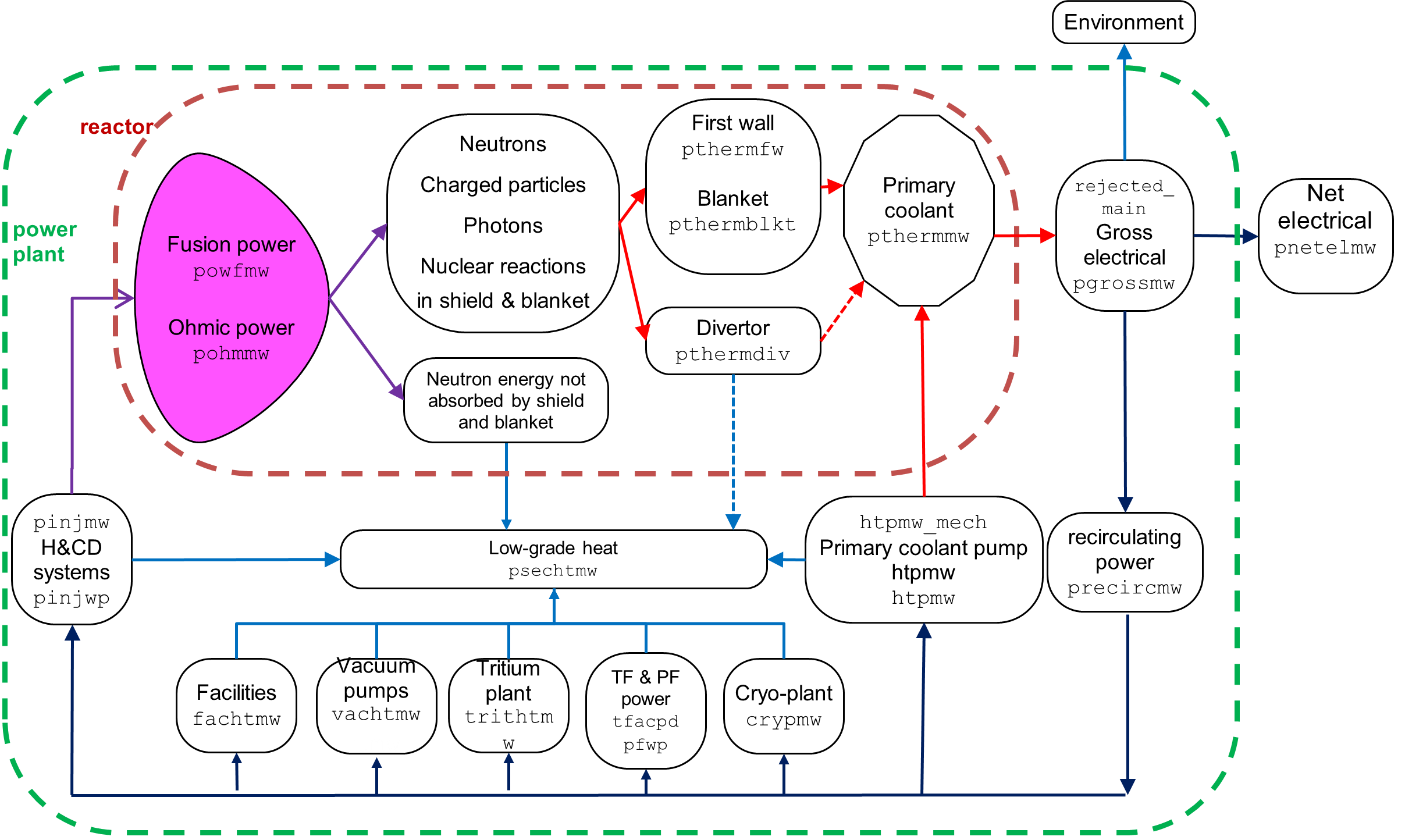
The primary sources of power are the fusion reactions themselves, ohmic power due to resistive heating within the plasma, and any auxiliary power provided for heating and current drive. The power carried by the fusion-generated neutrons is lost from the plasma, but is deposited in the surrounding material. A fraction falpha of the alpha particle power is assumed to stay within the plasma core to contribute to the plasma power balance. The sum of this core alpha power, any power carried by non-alpha charged particles, the ohmic power and any injected power, is converted into charged particle transport power ($P_{\mbox{loss}}$) plus core radiation power, as shown in the Figure. The core power balance calculation is turned on using constraint equation no. 2 (which should therefore always be used).

Bootstrap, Diamagnetic and Pfirsch-Schlüter Current Scalings

The fraction of the plasma current provided by the bootstrap effect can be either input into the code directly, or calculated using one of four methods, as summarised here. Note that methods ibss = 1-3 do not take into account the existence of pedestals, whereas the Sauter et al. scaling (ibss = 4) allows general profiles to be used.

ibss	Description
1	ITER scaling -- To use the ITER scaling method for the bootstrap current fraction. Set bscfmax to the maximum required bootstrap current fraction ($\leq 1$). This method is valid at high aspect ratio only.
2	General scaling[^15] -- To use a more general scaling method, set bscfmax to the maximum required bootstrap current fraction ($\leq 1$).
3	Numerically fitted scaling15 -- To use a numerically fitted scaling method, valid for all aspect ratios, set bscfmax to the maximum required bootstrap current fraction ($\leq 1$).
4	Sauter, Angioni and Lin-Liu scaling16 17 -- Set bscfmax to the maximum required bootstrap current fraction ($\leq 1$).

Fixed Bootstrap Current

Direct input -- To input the bootstrap current fraction directly, set bscfmax to $(-1)$ times the required value (e.g. -0.73 sets the bootstrap faction to 0.73).

The diamagnetic current fraction $f_{dia}$ is strongly related to $\beta$ and is typically small, hence it is usually neglected. For high $\beta$ plasmas, such as those at tight aspect ratio, it should be included and two scalings are offered. If the diamagnetic current is expected to be above one per cent of the plasma current, a warning is issued to calculate it.

idia = 0 Diamagnetic current fraction is zero.

idia = 1 Diamagnetic current fraction is calculated using a fit to spherical tokamak calculations by Tim Hender:

$$f_{dia} = \frac{\beta}{2.8}$$

idia = 2 Diamagnetic current fraction is calculated using a SCENE fit for all aspect ratios:

$$f_{dia} = 0.414 \space \beta \space (\frac{0.1 q_{95}}{q_0} + 0.44)$$

A similar scaling is available for the Pfirsch-Schlüter current fraction $f_{PS}$. This is typically smaller than the diamagnetic current, but is negative.

ips = 0 Pfirsch-Schlüter current fraction is set to zero.

ips = 1 Pfirsch-Schlüter current fraction is calculated using a SCENE fit for all aspect ratios:

$$f_{PS} = -0.09 \beta$$

There is no ability to input the diamagnetic and Pfirsch-Schlüter current directly. In this case, it is recommended to turn off these two scalings and to use the method of fixing the bootstrap current fraction.

L-H Power Threshold Scalings

Transitions from a standard confinement mode (L-mode) to an improved confinement regime (H-mode), called L-H transitions, are observed in most tokamaks. A range of scaling laws are available that provide estimates of the heating power required to initiate these transitions, via extrapolations from present-day devices. PROCESS calculates these power threshold values for the scaling laws listed in the table below, in routine pthresh.

For an H-mode plasma, use input parameter ilhthresh to select the scaling to use, and turn on constraint equation no. 15 with iteration variable no. 103 (flhthresh). By default, this will ensure that the power reaching the divertor is at least equal to the threshold power calculated for the chosen scaling, which is a necessary condition for H-mode.

For an L-mode plasma, use input parameter ilhthresh to select the scaling to use, and turn on constraint equation no. 15 with iteration variable no. 103 (flhthresh). Set lower and upper bounds for the f-value boundl(103) = 0.001 and boundu(103) = 1.0 to ensure that the power does not exceed the calculated threshold, and therefore the machine remains in L-mode.

ilhthresh	Name	Reference
1	ITER 1996 nominal	ITER Physics Design Description Document
2	ITER 1996 upper bound	D. Boucher, p.2-2
3	ITER 1996 lower bound
4	ITER 1997 excluding elongation	J. A. Snipes, ITER H-mode Threshold Database
5	ITER 1997 including elongation	Working Group, Controlled Fusion and Plasma Physics, 24th EPS conference, Berchtesgaden, June 1997, vol.21A, part III, p.961
6	Martin 2008 nominal	Martin et al, 11th IAEA Tech. Meeting
7	Martin 2008 95% upper bound	H-mode Physics and Transport Barriers, Journal
8	Martin 2008 95% lower bound	of Physics: Conference Series 123, 2008
9	Snipes 2000 nominal	J. A. Snipes and the International H-mode
10	Snipes 2000 upper bound	Threshold Database Working Group
11	Snipes 2000 lower bound	2000, Plasma Phys. Control. Fusion, 42, A299
12	Snipes 2000 (closed divertor): nominal
13	Snipes 2000 (closed divertor): upper bound
14	Snipes 2000 (closed divertor): lower bound
15	Hubbard 2012 L-I threshold scaling: nominal	Hubbard et al. (2012; Nucl. Fusion 52 114009)
16	Hubbard 2012 L-I threshold scaling: lower bound	[Hubbard et al. (2012; Nucl. Fusion 52 114009)](https://iopscience.iop.org/article/10.1088/0029-5515/52/11/114009
17	Hubbard 2012 L-I threshold scaling: upper bound	[Hubbard et al. (2012; Nucl. Fusion 52 114009)](https://iopscience.iop.org/article/10.1088/0029-5515/52/11/114009
18	Hubbard 2017 L-I threshold scaling	Hubbard et al. (2017; Nucl. Fusion 57 126039)
19	Martin 2008 aspect ratio corrected nominal	Martin et al (2008; J Phys Conf, 123, 012033)
20	Martin 2008 aspect ratio corrected 95% upper bound	Takizuka et al. (2004; Plasma Phys. Contol. Fusion, 46, A227)
21	Martin 2008 aspect ratio corrected 95% lower bound

Ignition

Switch ignite can be used to denote whether the plasma is ignited, i.e. fully self-sustaining without the need for any injected auxiliary power during the burn. If ignite = 1, the calculated injected power does not contribute to the plasma power balance, although the cost of the auxiliary power system is taken into account (the system is then assumed to be required to provide heating and/or current drive during the plasma start-up phase only). If ignite = 0, the plasma is not ignited, and the auxiliary power is taken into account in the plasma power balance during the burn phase. An ignited plasma will be difficult to control and is unlikely to be practical. This option is not recommended.

Other Plasma Physics Options

Neo-Classical Correction Effects

Neo-classical trapped particle effects are included in the calculation of the plasma resistance and ohmic heating power in subroutine pohm, which is called by routine physics. The scaling used is only valid for aspect ratios between 2.5 and 4, and it is possible for the plasma resistance to be incorrect or even negative if the aspect ratio is outside this range. An error is reported if the calculated plasma resistance is negative.

Inverse Quadrature in $\tau_E$ Scaling Laws

Switch iinvqd determines whether the energy confinement time scaling laws due to Kaye-Goldston (isc = 5) and Goldston (isc = 9) should include an inverse quadrature scaling with the Neo-Alcator result (isc = 1). A value iinvqd = 1includes this scaling.

Plasma-Wall Gap

The region directly outside the last closed flux surface of the core plasma is known as the scrape-off layer, and contains no structural material. Plasma entering this region is not confined and is removed by the divertor. PROCESS treats the scrape-off layer merely as a gap. Switch iscrp determines whether the inboard and outboard gaps should be calculated as 10% of the plasma minor radius (iscrp = 0), or set equal to the input values scrapli and scraplo (iscrp = 1).

---

1. J.D. Galambos, 'STAR Code : Spherical Tokamak Analysis and Reactor Code', Unpublished internal Oak Ridge document. ↩↩

2. H. Zohm et al, 'On the Physics Guidelines for a Tokamak DEMO', FTP/3-3, Proc. IAEA Fusion Energy Conference, October 2012, San Diego ↩

3. Y. Sakamoto, 'Recent progress in vertical stability analysis in JA', Task meeting EU-JA #16, Fusion for Energy, Garching, 24--25 June 2014 ↩

4. H.S. Bosch and G.M. Hale, 'Improved Formulas for Fusion Cross-sections and Thermal Reactivities', Nuclear Fusion 32 (1992) 611 ↩↩

5. J. Johner, 'Helios: A Zero-Dimensional Tool for Next Step and Reactor Studies', Fusion Science and Technology 59 (2011) 308--349 ↩

6. M. Bernert et al. Plasma Phys. Control. Fus. 57 (2015) 014038 ↩

7. N.A. Uckan and ITER Physics Group, 'ITER Physics Design Guidelines: 1989', ITER Documentation Series, No. 10, IAEA/ITER/DS/10 (1990) ↩↩↩↩↩

8. T. C. Hender et al., 'Physics Assessment for the European Reactor Study', AEA Fusion Report AEA FUS 172 (1992) ↩↩↩↩↩↩

9. D.J. Ward, 'PROCESS Fast Alpha Pressure', Work File Note F/PL/PJK/PROCESS/CODE/050 ↩↩

10. H. Lux, R. Kemp, D.J. Ward, M. Sertoli, 'Impurity radiation in DEMO systems modelling', Fus. Eng. | Des. 101, 42-51 (2015) ↩↩

11. Albajar, Nuclear Fusion 41 (2001) 665 ↩

12. Fidone, Giruzzi and Granata, Nuclear Fusion 41 (2001) 1755 ↩

13. N.A. Uckan, Fusion Technology 14 (1988) 299 ↩

14. W.M. Nevins, 'Summary Report: ITER Specialists' Meeting on Heating and Current Drive', ITER-TN-PH-8-4, 13--17 June 1988, Garching, FRG ↩

15. H.R. Wilson, Nuclear Fusion 32 (1992) 257 ↩

16. O. Sauter, C. Angioni and Y.R. Lin-Liu, Physics of Plasmas 6 (1999) 2834 ↩

17. O. Sauter, C. Angioni and Y.R. Lin-Liu, Physics of Plasmas 9 (2002) 5140 ↩

18. M. Kovari, R. Kemp, H. Lux, P. Knight, J. Morris, D.J. Ward, '“PROCESS”: A systems code for fusion power plants—Part 1: Physics' Fusion Engineering and Design 89 (2014) 3054–3069 ↩